A result may look impressive and still be irrelevant. “Six accepted” means little until we know how many received the offer, who they were, and what happened afterward. Analyzing experiments combines correct calculations, contextual reading, and caution about alternative explanations [R09][R17].
Identify the question and data type first
Qualitative data describe behavior, obstacles, motives, and accounts. Quantitative data count events, times, and standardized responses. They are complementary: a rate tells us how much occurred in a sample, while observation may help explain why. A small qualitative study should not be treated as a precise estimate for an entire population [R17].
Clean and trace data before calculating
Check duplicate IDs, dates, eligibility rules, missing events, protocol changes, and observations from different conditions. Decide how to treat incomplete records and document the choice. Do not fill missing values by assuming every missing result was a success or a failure. See documenting experiment results for the original record.
Quantitative example: ten eligible restaurants
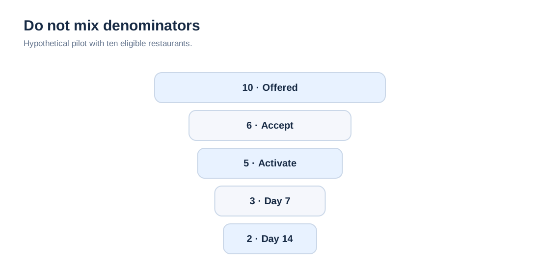
Imagine a fully hypothetical pilot using the same offer and a defined manager group. The offer went to 10 eligible venues; 6 agreed; 5 activated the service; 3 were still using it on day seven; 2 on day fourteen. No payment was requested during this trial.
| Event | Count | Explicit denominator | Descriptive rate |
|---|---|---|---|
| Accepted pilot offer | 6 | 10 eligible venues offered | 60% |
| Activated after accepting | 5 | 6 who accepted | 83.3% |
| Used on day 7 | 3 | 5 who activated | 60% |
| Used on day 14 | 2 | 5 who activated | 40% |
| Payment recorded | 0 | No paid offer was presented | Not computable as a purchase conversion rate |
Changing the denominator changes the question: two active users on day fourteen are 40% of activated users, or 20% of all eligible venues offered the pilot. Both figures can be correct with proper labels. Neither establishes a representative population rate from a convenience sample.
When numbers are small
With ten cases, one person can move the acceptance percentage by ten points. Do not automatically extrapolate an exact estimate to thousands of restaurants. Confidence intervals can help when sampling design and inference assumptions support them; they do not turn a biased convenience sample into a probability sample [R15]. Statistical significance cannot be inferred just because one percentage is larger: hypotheses, design, sample size, and appropriate analysis are required.
To judge how much confidence the sample can support, review how to evaluate evidence, bias, and alternative explanations. Computing a percentage correctly cannot repair an unsuitable participant selection process.
Analyze what people said and did
If users drop out, group observations by themes: setup time, duplicate work, confusing notifications, technical outages. Retain quotes and behavior that contradict the dominant themes. Do not force all responses into categories invented afterward to validate the preferred idea. Ask who observed the sessions, how themes were coded, and whether another analyst might interpret them similarly [R09].
Comparison and causality
Comparing Monday activations with Friday activations may mix weekday effects, staff availability, and sales-team behavior. Two variables moving together does not establish causation. Estimating an effect calls for comparable conditions, suitable allocation, and appropriate analysis; exploring possible causes may benefit more from qualitative work than premature A/B testing [R11][R17]. Review experiment bias.
From result to conclusion
The starting hypothesis claimed five of ten venues would accept: we observed six, so the acceptance threshold was reached in this sample. Yet only two of five activated venues remained active on day fourteen; calling retention sufficient would be premature. Because nobody received a paid offer, there is no direct evidence of willingness to pay. A sound conclusion states scope, uncertainty, and the next question.
When that next question requires changing the offer, hypothesis, or test, use the Design–Test Loop to iterate with evidence. Do not rerun the same experiment until it looks favorable; record what you learned and what changed.
Use a decision tree to turn favorable, unfavorable, and inconclusive evidence into actions without treating evidence as certainty.
What you should have by the end: cleaned data, calculations with denominators, qualitative findings, and a conclusion proportional to the evidence. Main sources: [R09], [R11], [R15], [R17].
Bibliography and references
- [R09] GOV.UK Service Manual. Analyse a research session. https://www.gov.uk/service-manual/user-research/analyse-a-research-session — Diferenciar observaciones e interpretaciones.
- [R17] Nielsen Norman Group. Quantitative vs. Qualitative Usability Testing. https://www.nngroup.com/articles/quant-vs-qual/ — Investigación cualitativa y cuantitativa.
- [R15] NIST/SEMATECH e-Handbook. Confidence intervals. https://www.itl.nist.gov/div898/handbook/prc/section2/prc241.htm — Incertidumbre para estimar proporciones.
- [R11] NIST/SEMATECH e-Handbook. Choosing an experimental design. https://itl.nist.gov/div898/handbook/pri/section3/pri3.htm — Variables, aleatorización, factores de confusión y diseños comparativos.